44 pie chart excel labels
Only Display Some Labels On Pie Chart - Excel Help Forum Only Display Some Labels On Pie Chart. I have a pie chart that contains over 50 categories (Yes, I know pie charts shouldn't be used for that many things) but I want to only display labels for maybe the top 5 values or any label with a value >10. This is because there are a few standout values but I want all the other values to remain in the ... Pie Chart - legend missing one category (edited to include spreadsheet ... Re: Pie Chart - legend missing one category (edited to include spreadsheet) Excel is getting confused by your merged cells. If possible, unmerge the cells, and link the label to a single cell. If you don't want to unmerge, then change the label refs in the series formula for the chart. Click on the pie chart, and in the formula bar, change the ...
How to show percentage in pie chart in Excel? - ExtendOffice Please do as follows to create a pie chart and show percentage in the pie slices. 1. Select the data you will create a pie chart based on, click Insert > I nsert Pie or Doughnut Chart > Pie. See screenshot: 2. Then a pie chart is created. Right click the pie chart and select Add Data Labels from the context menu. 3.

Pie chart excel labels
Creating Pie Chart and Adding/Formatting Data Labels (Excel) Creating Pie Chart and Adding/Formatting Data Labels (Excel) How to display leader lines in pie chart in Excel? - ExtendOffice To display leader lines in pie chart, you just need to check an option then drag the labels out. 1. Click at the chart, and right click to select Format Data Labels from context menu. 2. In the popping Format Data Labels dialog/pane, check Show Leader Lines in the Label Options section. See screenshot: 3. How to Show Percentage in Pie Chart in Excel? - GeeksforGeeks Show percentage in a pie chart: The steps are as follows : Select the pie chart. Right-click on it. A pop-down menu will appear. Click on the Format Data Labels option. The Format Data Labels dialog box will appear. In this dialog box check the "Percentage" button and uncheck the Value button. This will replace the data labels in pie chart ...
Pie chart excel labels. Chart Legend / Data Labels In Pie Chart - MrExcel Message Board Add the data labels. Then, right click on any data label to select all the data labels for that series and select Format Data Labels... From the Label Options tab, in the Label Contains section, select the 'Series Name' checkbox. The above applies to Excel 2007. Excel 2003 supports the same capability though the dialog box choices may be different. excel - Positioning data labels in pie chart - Stack Overflow Sub tester () Dim se As Series Set se = Totalt.ChartObjects ("Inosa gule").Chart.SeriesCollection ("Grøn pil") se.ApplyDataLabels With se.DataLabels .NumberFormat = "0,0 %" With .Format.Fill .ForeColor.RGB = RGB (255, 255, 255) .Transparency = 0.15 End With .Position = xlLabelPositionCenter End With End Sub How to Rotate Pie Chart in Excel? - WallStreetMojo Move the cursor to the chart area to select the pie chart. Step 5: Click on the Pie chart and select the 3D chart, as shown in the figure, and develop a 3D pie chart. Step 6: In the next step, change the title of the chart and add data labels to it. Step 7: To rotate the pie chart, click on the chart area. Pie Chart Best Fit Labels Overlapping - VBA Fix - Microsoft Tech Community I created attached Pie chart in Excel with 31 points and all labels are readable and perfectly placed. It is created from few clicks without VBA using data visualization tool in Excel. Data Visualization Tool For Excel Data Visualization Tool For Google Sheets It has auto cluttering effect to adjust according to your data size.
Formatting data labels and printing pie charts on Excel for Mac 2019 ... Here's a work around I found for printing pie charts. Still can't find a solution for formatting the data labels. 1. When printing a pie chart from Excel for mac 2019, MS instructions are to select the chart only, on the worksheet > file > print. Excel is supposed to print the chart only (not the data ) and automatically fit it onto one page. How to plot a pie chart in Excel | Basic Excel Tutorial NOTE. 1. On your computer, open the worksheet you want to create a pie chart. 2. In your spreadsheet, select the range of data you want to use for your pie chart. 3. On the main menu ribbon, click on the Insert tab. 4. Here you will see different types of charts, click on the Pie chart icon drop-down arrow. Pie Chart in Excel | How to Create Pie Chart - EDUCBA Pie Chart in Excel is used for showing the completion or main contribution of different segments out of 100%. It is like each value represents the portion of the Slice from the total complete Pie. For Example, we have 4 values A, B, C and D. How to eliminate zero value labels in a pie chart - MrExcel Message Board However you can hide the 0% using custom number formatting. Right click the label and select Format Data Labels. Then select the Number tab and then Custom from the Categories. Enter. 0%; [White] [=0]General;General. in the Type box. This will set the font colour to white if a label has a value of zero.
How to Create a Pie Chart in Excel | Smartsheet To create a pie chart in Excel 2016, add your data set to a worksheet and highlight it. Then click the Insert tab, and click the dropdown menu next to the image of a pie chart. Select the chart type you want to use and the chosen chart will appear on the worksheet with the data you selected. Microsoft Excel Tutorials: Add Data Labels to a Pie Chart - Home and Learn To add the numbers from our E column (the viewing figures), left click on the pie chart itself to select it: The chart is selected when you can see all those blue circles surrounding it. Now right click the chart. You should get the following menu: From the menu, select Add Data Labels. New data labels will then appear on your chart: How to Customize Your Excel Pivot Chart Data Labels - dummies The Data Labels command on the Design tab's Add Chart Element menu in Excel allows you to label data markers with values from your pivot table. When you click the command button, Excel displays a menu with commands corresponding to locations for the data labels: None, Center, Left, Right, Above, and Below. None signifies that no data labels should be added to the chart and Show signifies ... Pie Chart in Excel - Inserting, Formatting, Filters, Data Labels Right click on the Data Labels on the chart. Click on Format Data Labels option. Consequently, this will open up the Format Data Labels pane on the right of the excel worksheet. Mark the Category Name, Percentage and Legend Key. Also mark the labels position at Outside End. This is how the chark looks. Formatting the Chart Background, Chart Styles
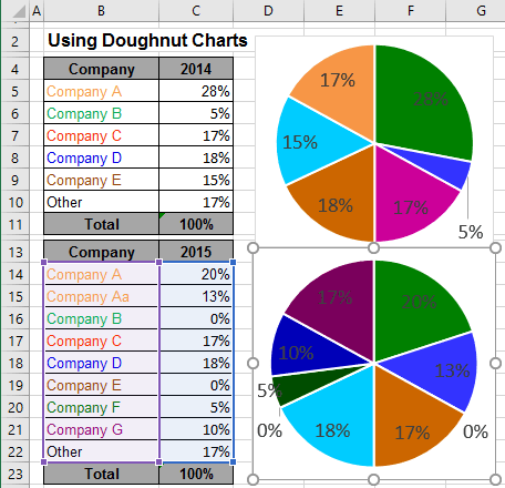
Using Pie Charts and Doughnut Charts in Excel
Excel custom pie chart labels - Microsoft Community Excel custom pie chart labels I have a data set like this (basically form output): I want to use a pivot table to make a pie chart out of this. I want each of the pieces of the pie to contain the number of entries and between parentheses the percentage. So in the "Yes" piece, there should be '3 (33%)'.
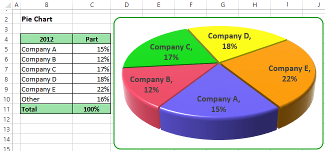
Excel 3-D Pie Charts - Microsoft Excel 2013
Excel 2010 pie chart data labels in case of "Best Fit" Based on my tested in Excel 2010, the data labels in the "Inside" or "Outside" is based on the data source. If the gap between the data is big, the data labels and leader lines is "outside" the chart. And if the gap between the data is small, the data labels and leader lines is "inside" the chart. Regards, George Zhao. TechNet Community Support.
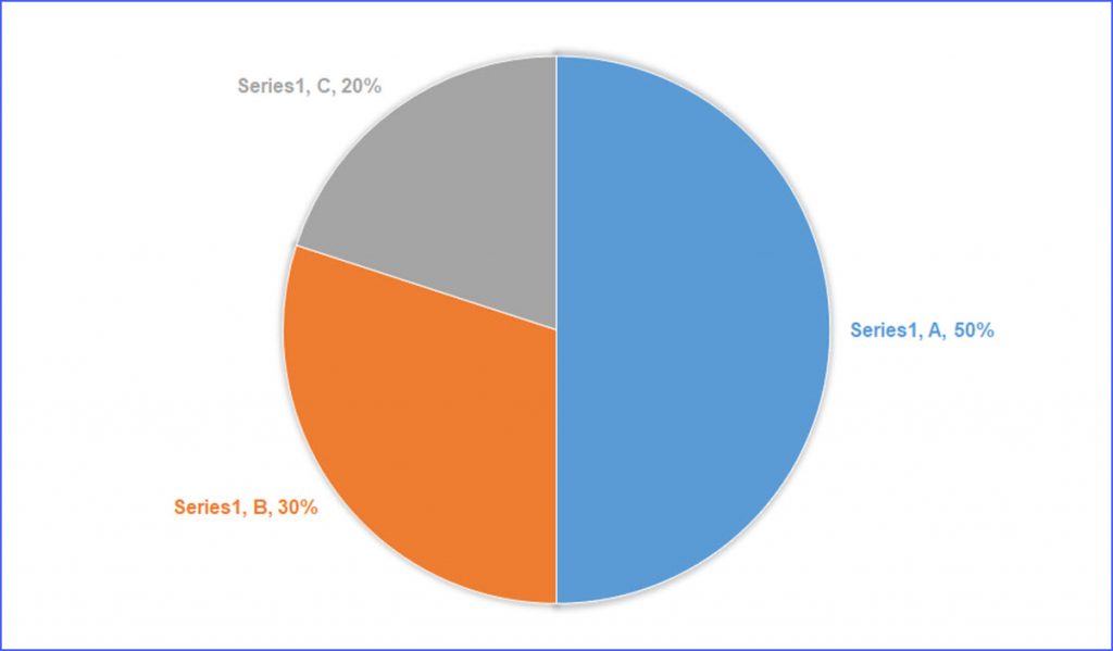
How to Make Labels the Same Color as the Pies in Pie Chart - ExcelNotes
How to Insert Axis Labels In An Excel Chart | Excelchat We will go to Chart Design and select Add Chart Element Figure 6 - Insert axis labels in Excel In the drop-down menu, we will click on Axis Titles, and subsequently, select Primary vertical Figure 7 - Edit vertical axis labels in Excel Now, we can enter the name we want for the primary vertical axis label.
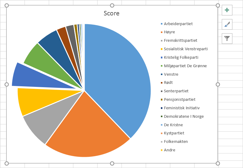
13. Extract a slice from the pie – bioST@TS
How to Create and Format a Pie Chart in Excel - Lifewire Select the plot area of the pie chart. Right-click the chart. Select Add Data Labels . Select Add Data Labels. In this example, the sales for each cookie is added to the slices of the pie chart. Change Colors When a chart is created in Excel, or whenever an existing chart is selected, two additional tabs are added to the ribbon.
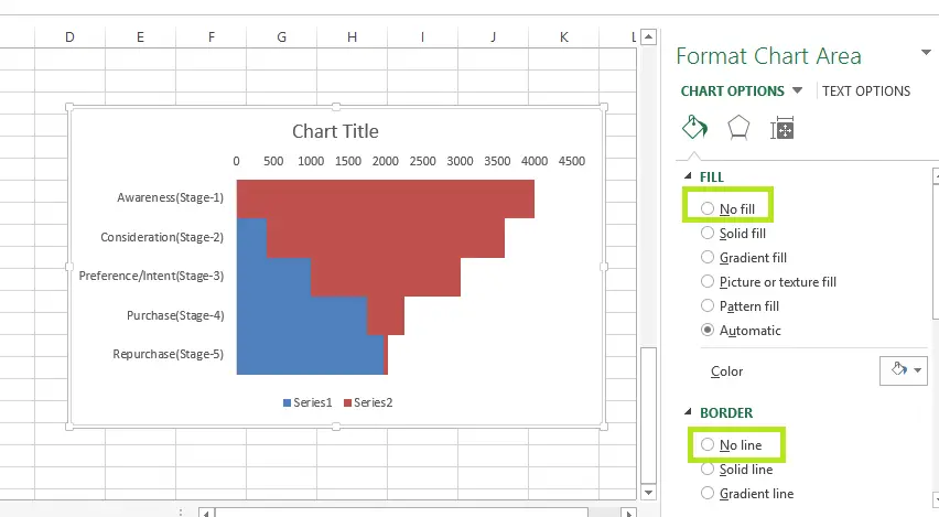
Funnel Chart in Excel - DataScience Made Simple
Multiple data labels (in separate locations on chart) You can do it in a single chart. Create the chart so it has 2 columns of data. At first only the 1 column of data will be displayed. Move that series to the secondary axis. You can now apply different data labels to each series. Attached Files 819208.xlsx (13.8 KB, 263 views) Download Cheers Andy Register To Reply

How to Create a Pie Chart in Microsoft Excel
Everything You Need to Know About Pie Chart in Excel - SpreadsheetWeb How to Make a Pie Chart in Excel. Start with selecting your data in Excel. If you include data labels in your selection, Excel will automatically assign them to each column and generate the chart. Go to the INSERT tab in the Ribbon and click on the Pie Chart icon to see the pie chart types. Click on the desired chart to insert.
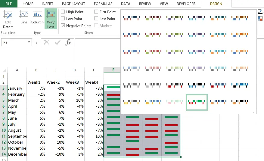
Win Loss Chart in Excel - DataScience Made Simple
Pie of Pie Chart in Excel - Inserting, Customizing, Formatting Inserting a Pie of Pie Chart. Let us say we have the sales of different items of a bakery. Below is the data:-. To insert a Pie of Pie chart:-. Select the data range A1:B7. Enter in the Insert Tab. Select the Pie button, in the charts group. Select Pie of Pie chart in the 2D chart section.
Post a Comment for "44 pie chart excel labels"