43 data labels excel 2013
Data Labels auto fill [SOLVED] - excelforum.com Re: Data Labels auto fill. Hi Fawnlemur, To add the data label for %age you can follow these steps:- When you will click on chart then 2 contextual tabs will get appear, then click on Design tab, go to in the Chart layout's group, click on "Add Chart Element", where you will see the "Data Label" option when you will click on "Data Label option ... How to add data labels from different column in an Excel chart? Right click the data series in the chart, and select Add Data Labels > Add Data Labels from the context menu to add data labels. 2. Click any data label to select all data labels, and then click the specified data label to select it only in the chart. 3.
Add or remove data labels in a chart - support.microsoft.com Right-click the data series or data label to display more data for, and then click Format Data Labels. Click Label Options and under Label Contains, select the Values From Cells checkbox. When the Data Label Range dialog box appears, go back to the spreadsheet and select the range for which you want the cell values to display as data labels.

Data labels excel 2013
Values From Cell: Missing Data Labels Option in Excel 2013? When a chart created in 2013 using the "Values from Cell" data label option is opened with any earlier version of Excel, the data labels will show as " [CELLRANGE]". If you want to ensure that data labels survive different generations of Excel, you need to revert to the old technique: Insert data labels Edit each individual data label How to Print Labels from Excel - Lifewire Choose Start Mail Merge > Labels . Choose the brand in the Label Vendors box and then choose the product number, which is listed on the label package. You can also select New Label if you want to enter custom label dimensions. Click OK when you are ready to proceed. Connect the Worksheet to the Labels How to Add Data Tables to Charts in Excel 2013 - dummies To add a data table to your selected chart and position and format it, click the Chart Elements button next to the chart and then select the Data Table check box before you select one of the following options on its continuation menu: With Legend Keys to have Excel draw the table at the bottom of the chart, including the color keys used in the ...
Data labels excel 2013. Excel: Chart Labels in Excel 2013 - Excel Articles Excel Excel 2013 introduces a new feature where the chart labels can come from other cells on the worksheet. In the Figure below, formulas in column C build a label to identify the largest and second largest sales amount. ... Click the 3-Column chart icon in the Format Data Labels Task Pane. Click on Label Options. Checkmark Value From Cells ... How to create Custom Data Labels in Excel Charts Create the chart as usual. Add default data labels. Click on each unwanted label (using slow double click) and delete it. Select each item where you want the custom label one at a time. Press F2 to move focus to the Formula editing box. Type the equal to sign. Now click on the cell which contains the appropriate label. chandoo.org › wp › change-data-labels-in-chartsHow to Change Excel Chart Data Labels to Custom Values? May 05, 2010 · Now, click on any data label. This will select “all” data labels. Now click once again. At this point excel will select only one data label. Go to Formula bar, press = and point to the cell where the data label for that chart data point is defined. Repeat the process for all other data labels, one after another. See the screencast. Adding Data Labels to Your Chart (Microsoft Excel) To add data labels in Excel 2013 or Excel 2016, follow these steps: Activate the chart by clicking on it, if necessary. Make sure the Design tab of the ribbon is displayed. (This will appear when the chart is selected.) Click the Add Chart Element drop-down list. Select the Data Labels tool.
› excel-charts-title-axis-legendExcel charts: add title, customize chart axis, legend and ... Oct 29, 2015 · For example, this is how we can add labels to one of the data series in our Excel chart: For specific chart types, such as pie chart, you can also choose the labels location. For this, click the arrow next to Data Labels, and choose the option you want. To show data labels inside text bubbles, click Data Callout. How to change data displayed on ... Custom Chart Data Labels In Excel With Formulas Follow the steps below to create the custom data labels. Select the chart label you want to change. In the formula-bar hit = (equals), select the cell reference containing your chart label's data. In this case, the first label is in cell E2. Finally, repeat for all your chart laebls. Creating a chart with dynamic labels - Microsoft Excel 2013 Excel 2013 365 2016. This tip shows how to create dynamically updated chart labels that depend on value or other cells. ... For all labels: on the Format Data Labels task pane, in the Label Options, in the Label Contains group, check Value From Cells and then choose cells: Custom Chart Labels Using Excel 2013 | MyExcelOnline View the Benchmark Chart using Excel 2013. DOWNLOAD EXCEL WORKBOOK. STEP 1: We added a % Variance column in our data and inserted symbols to show a negative and positive variance. ** You can see the tutorial of how this is done here **. STEP 2: In our graph we need to select the Sales chart and Right Click and choose Add Data Labels.
Excel tutorial: How to use data labels Generally, the easiest way to show data labels to use the chart elements menu. When you check the box, you'll see data labels appear in the chart. If you have more than one data series, you can select a series first, then turn on data labels for that series only. You can even select a single bar, and show just one data label. data labels in chart - excel 2013 | MrExcel Message Board Hi I have 3 data labels in column chart. I changed the shape of these labels to Oval Callout. if I select one of them to format, then they will be all selected as well. Which is good and understandable. But how can I move them all at same time. Now when I click on one of them then they will all... How to Add Data Labels in Excel - Excelchat | Excelchat How to Add Data Labels In Excel 2013 And Later Versions In Excel 2013 and the later versions we need to do the followings; Click anywhere in the chart area to display the Chart Elements button Figure 5. Chart Elements Button Click the Chart Elements button > Select the Data Labels, then click the Arrow to choose the data labels position. Figure 6. › format-data-labels-in-excelFormat Data Labels in Excel- Instructions - TeachUcomp, Inc. Nov 14, 2019 · Then select the “Format Data Labels…” command from the pop-up menu that appears to format data labels in Excel. Using either method then displays the “Format Data Labels” task pane at the right side of the screen. Format Data Labels in Excel- Instructions: A picture of the “Format Data Labels” task pane in Excel.

Excel 2013 Tutorial Formatting Data Labels Microsoft Training Lesson 28.6 - YouTube
How to Data Labels in a Line Graph in Excel 2013 - YouTube Want to insert Data Labels in a line graph in Microsoft® Excel 2013? Follow the easy steps shown in this video. Content in this video is provided on an ""as ...

Excel chart not printing correctly - i have a simple excel file (office
Excel Data Labels - Microsoft Community Excel Data Labels. Hello! I created a chart and linked the data labels to a series of cells, as 2013 allows in Value From Cells option. fyi: The data labels are names of individuals, and the data points (x,y numbers) are in two other columns. I create this to use as a template (but not Saved As a "template" proper).
DPlot Graph Software for Scientists and Engineers
› excel › how-to-add-total-dataHow to Add Total Data Labels to the Excel Stacked Bar Chart Apr 03, 2013 · Step 4: Right click your new line chart and select “Add Data Labels” Step 5: Right click your new data labels and format them so that their label position is “Above”; also make the labels bold and increase the font size. Step 6: Right click the line, select “Format Data Series”; in the Line Color menu, select “No line”

Excel 3-D Pie Charts
How to Add Data Labels to your Excel Chart in Excel 2013 Data labels show the values next to the corresponding chart element, for instance a percentage next to a piece from a pie chart, or a total value next to a column in a column chart. You can choose...
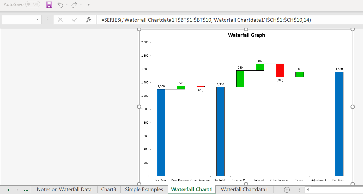
Waterfall Chart Templates (Excel 2010 and 2013) – Edward Bodmer – Project and Corporate Finance
Adding rich data labels to charts in Excel 2013 | Microsoft 365 Blog You can do this by adjusting the zoom control on the bottom right corner of Excel's chrome. Then, select the value in the data label and hit the right-arrow key on your keyboard. The story behind the data in our example is that the temperature increased significantly on Wednesday and that appeared to help drive up business at the lemonade stand.

How to Add Data Labels to an Excel 2010 Chart - dummies
Tip - Adding rich data labels to charts in Excel 2013 You can do this by adjusting the zoom control on the bottom right corner of Excel's chrome. Then, select the value in the data label and hit the right-arrow key on your keyboard. The story behind the data in our example is that the temperature increased significantly on Wednesday and that appeared to help drive up business at the lemonade stand.
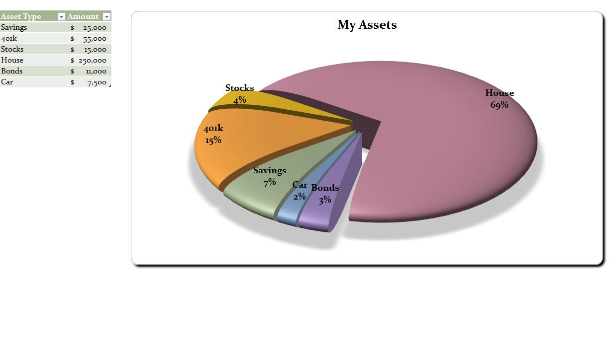
Excel Pie Chart | Pie Chart Excel
Values From Cell: Missing Data Labels Option in Excel 2013? 8. May 27, 2015. #1. Ive inherited a Powerpoin with an embedded Excel chart and data sheet. The graph in Powerpoint shows several instances of a value [CellRange]. Im trying to figure out where its "trying" to pull its data from and I think because the data is not in a contiguous range its having trouble. A couple articles refer to formatting ...
35 Label Definition Excel - Labels For Your Ideas
How to hide zero data labels in chart in Excel? - ExtendOffice Note: In Excel 2013, you can right click the any data label and select Format Data Labels to open the Format Data Labels pane; then click Number to expand its option; next click the Category box and select the Custom from the drop down list, and type #"" into the Format Code text box, and click the Add button.

How to Create Multi-Category Chart in Excel - Excel Board
Move data labels - support.microsoft.com Right-click the selection > Chart Elements > Data Labels arrow, and select the placement option you want. Different options are available for different chart types. For example, you can place data labels outside of the data points in a pie chart but not in a column chart.

Format Data Labels in Excel- Instructions - TeachUcomp, Inc.
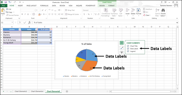
› excel_data_analysis › excelExcel Data Analysis - Data Visualization - tutorialspoint.com Data Labels. Excel 2013 and later versions provide you with various options to display Data Labels. You can choose one Data Label, format it as you like, and then use Clone Current Label to copy the formatting to the rest of the Data Labels in the chart. The Data Labels in a chart can have effects, varying shapes and sizes.
MS Excel 2013: Display the fields in the Values Section in a single column in a pivot table
Custom Data Labels with Colors and Symbols in Excel Charts - [How To] Step 4: Select the data in column C and hit Ctrl+1 to invoke format cell dialogue box. From left click custom and have your cursor in the type field and follow these steps: Press and Hold ALT key on the keyboard and on the Numpad hit 3 and 0 keys. Let go the ALT key and you will see that upward arrow is inserted.

Enable or Disable Excel Data Labels at the click of a button - How To - PakAccountants.com
powerbi.microsoft.com › en-us › blogPower BI April 2021 Feature Summary Apr 16, 2021 · Welcome to the first Power BI feature summary of the Spring! In this update we have an exciting new preview for the Power Automate visual! Also, the ongoing previews (Small Multiples and DirectQuery for Power BI datasets and Azure Analysis Services) are getting some new features. Next to that, we are presenting huge improvements to the shapes in Power BI Desktop and we are introducing a new ...

How to Create a Pie Chart in Microsoft Excel
Quick Tip: Excel 2013 offers flexible data labels | TechRepublic right-click and choose Insert Data Label Field. In the next dialog, select [Cell] Choose Cell. When Excel displays the source dialog, click the cell that contains the MIN () function, and click OK....

How to Create a Chart in Microsoft Excel - TechSupport
support.microsoft.com › en-us › officeTutorial: Import Data into Excel, and Create a Data Model In the next tutorial, Extend Data Model relationships using Excel 2013, Power Pivot, and DAX, you build on what you learned here, and step through extending the Data Model using a powerful and visual Excel add-in called Power Pivot. You also learn how to calculate columns in a table, and use that calculated column so that an otherwise unrelated ...
Post a Comment for "43 data labels excel 2013"