43 pivot table excel row labels side by side
Create a matrix visual in Power BI - Power BI | Microsoft Docs When you turn on Row subtotals and add a label, Power BI also adds a row, and the same label, for the grand total value. To format your grand total, select the format option for Row grand total. If you want to turn subtotals and the grand total off, in the format section of the visualizations pane, expand the Row subtotals card. Autofilling rows based on a range on another tab : excel This table is turned into a small summary table, a pivot table, and a pivot chart. Using the wonderful resources of stack overflow and Google, I finally got the next step. I now have a script in PowerShell that opens the workbook, runs the query, updates, the pivots, saves and closes, then emails this to the relevant managers.
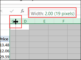
Overview of the Microsoft Office Ribbon - Computer Hope Side to Side - Scrolls from side-to-side to move between pages. Show. Ruler - Shows a ruler on the side of the document. Gridlines - Shows gridlines over the document. Navigation Pane - Shows a side pane with a search function. Zoom. Zoom - Increases the viewing size of the document. 100% - Displays the document at actual size.
Pivot table excel row labels side by side
3 Way Data Table Excel • AuditExcel.co.za A method to create three way data tables in Excel using the normal data table feature which normally only allows a two way data table. NEW: Get the templates from the Multi Variable Data Tables Tutorial. For updated video clips in structured Excel courses with practical example files, have a look at our MS Excel online training courses . You can even try the Free MS Excel tips and tricks course. Word Ribbon - View Tab - BetterSolutions.com New Window - Lets you create a new window of the active document. Arrange All - Tile all the open windows side by side on the screen. This will also maximises the application / document to a full screen. Split - Splits the current window into two parts. View Side by Side - Displays two documents side by side so they can be easily compared. If you have more than two documents open the "Compare ... How to convert rows to columns in Excel (transpose data) - Ablebits With the macro inserted in your workbook, perform the below steps to rotate your table: Open the target worksheet, press Alt + F8, select the TransposeColumnsRows macro, and click Run. Select the range that you want to transpose and click OK: Select the upper left cell of the destination range and click OK:
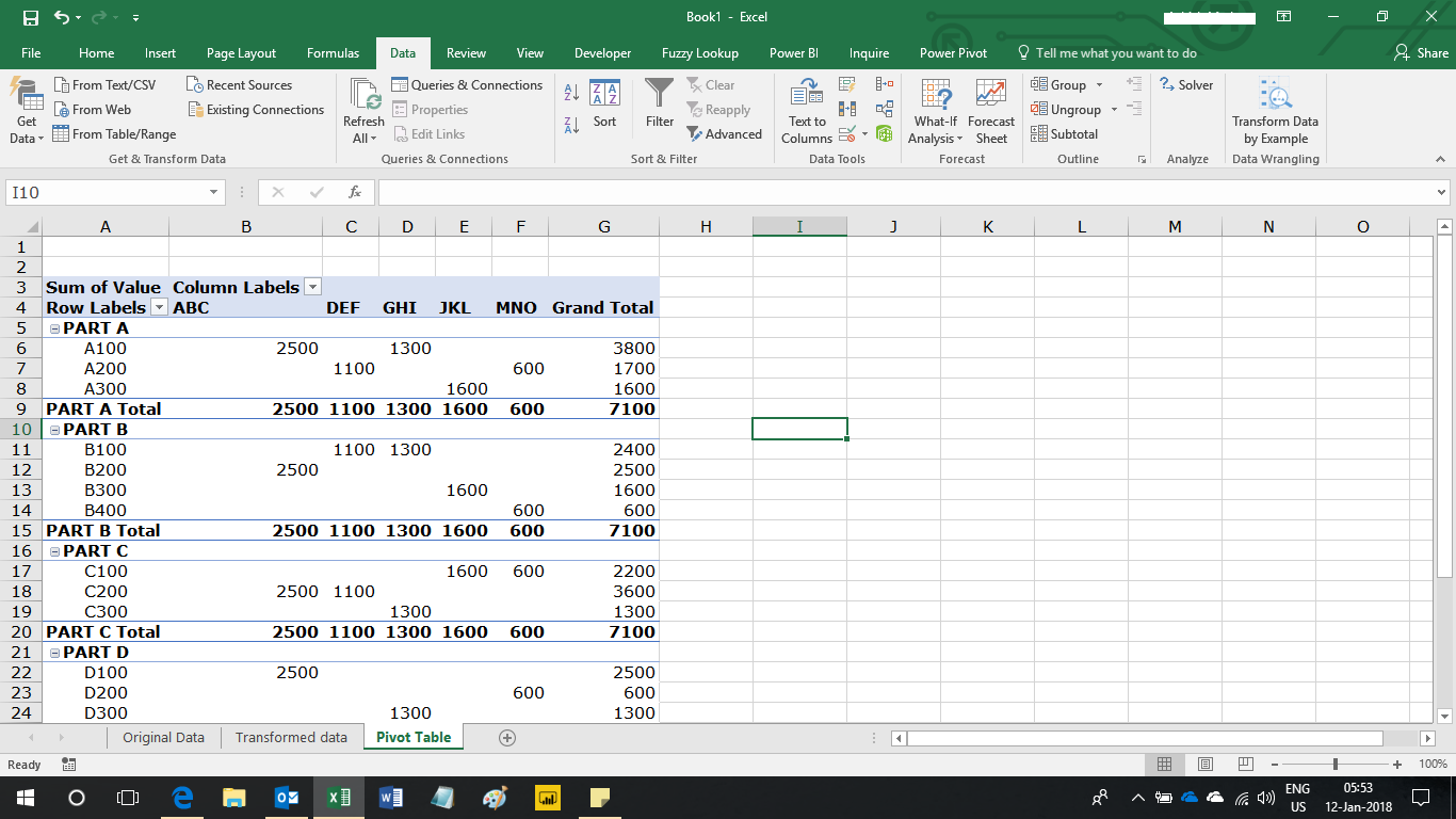
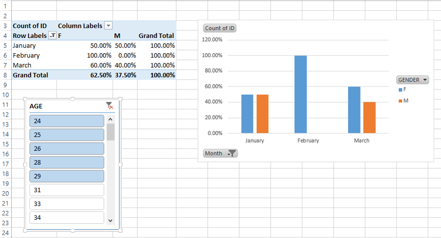
Pivot table excel row labels side by side. What Is An Excel Pivot Table And How To Create One - Software Testing Help Rows: Fields under Rows are the Row Labels displayed on the left side of the Pivot Table. Values: Mainly used to show the summarized numeric values. You can even add multiple fields in the same area like Region and City under Rows and you can check the resulting Pivot Table as shown in the diagram above if you want to remove a field from the table, just drag the field outside that area's section. Excel FAQ - Application and Files - Contextures Excel Tips Right-click the Excel icon in the Windows Taskbar, at the bottom of your screen. Then click the Close All Windows command. NOTE: This technique only works if the Taskbar has "Always, hide labels" as the setting for "Combine taskbar buttons: To change that setting, right-click the Taskbar, and click Taskbar Settings. Advanced Microsoft Excel 2016 | Cowley Community College Develop essential skills in Microsoft Excel 2016 to better consolidate, analyze, and report on data. This course provides expert instruction and hands-on exercises that will help you easily master analysis tools, PivotTables, conditional formatting, and other advanced features. 6 Weeks Access / 24 Course Hrs. Data Labels in Excel Pivot Chart (Detailed Analysis) Steps. Create the Pivot Table just like before and then drag the Region in the Axis area and Quantity in the Values area. Then add a Pivot Chart from the PivotTable Analyze tab. Next, you will notice that there is a data label option, but we want to add it manually from a range of cells.
Excel Pivot Tables That Automate Tasks You No Longer Have Time For How ... Automate Excel Pivot Table Reports. Excel pivot tables are an excellent way to display data to your end users. You can include a pivot table in an Excel report and use Automation to refresh the pivot table's source data in the report. In this example, you will export data to an Excel file with a pivot table. › excel-pivot-table-formatHow to Format Excel Pivot Table - Contextures Excel Tips Jun 22, 2022 · Video: Change Pivot Table Labels. Watch this short video tutorial to see how to make these changes to the pivot table headings and labels. Get the Sample File. No Macros: To experiment with pivot table styles and formatting, download the sample file. The zipped file is in xlsx format, and and does NOT contain any macros. 15 Excel Formulas, Keyboard Shortcuts & Tricks That'll Save ... - HubSpot NOTE: The following formulas apply to the latest version of Excel. If you're using a slightly older version of Excel, the location of each feature mentioned below might be slightly different. 1. SUM . All Excel formulas begin with the equals sign, =, followed by a specific text tag denoting the formula you'd like Excel to perform. Excel Easy: #1 Excel tutorial on the net 5 Pivot Tables: Pivot tables are one of Excel's most powerful features. A pivot table allows you to extract the significance from a large, detailed data set. 6 Tables: Master Excel tables and analyze your data quickly and easily. 7 What-If Analysis: What-If Analysis in Excel allows you to try out different values (scenarios) for formulas.
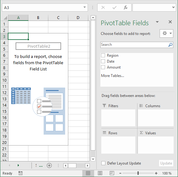
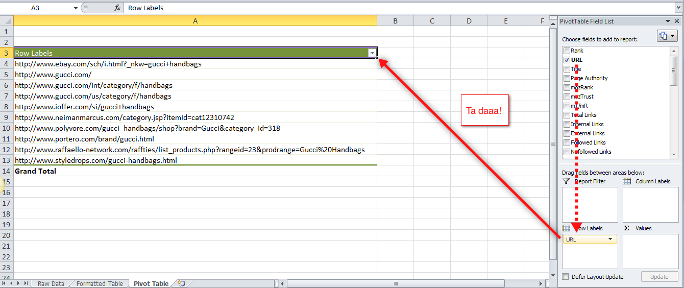
en.wikipedia.org › wiki › Pivot_tablePivot table - Wikipedia Pivot tables are not created automatically. For example, in Microsoft Excel one must first select the entire data in the original table and then go to the Insert tab and select "Pivot Table" (or "Pivot Chart"). The user then has the option of either inserting the pivot table into an existing sheet or creating a new sheet to house the pivot table. powerspreadsheets.com › excel-pivot-table-groupExcel Pivot Table Group: Step-By-Step Tutorial To Group Or ... In fact, as mentioned in Excel 2016 Pivot Table Data Crunching: Each time you create a new pivot table in Excel 2016, Excel automatically shares the pivot cache. Pivot Cache sharing has several benefits. Most notably, as I mention above, it reduces memory requirements and file size vs. the scenario where the Pivot Cache isn't shared. › createpivottableHow to Create a Pivot Table in Excel - Contextures Excel Tips Dec 14, 2021 · Create a Pivot Table in Excel. Follow these easy steps to create an Excel pivot table, so you can quickly summarize Excel data. Watch the short video to see the steps, or follow the written steps. Get the free workbook, to follow along. There's also an interactive pivot table below, that you can try, before you build your own! blog.hubspot.com › marketing › how-to-create-pivotHow to Create a Pivot Table in Excel: A Step-by-Step Tutorial Dec 31, 2021 · After you've completed Step 3, Excel will create a blank pivot table for you. Your next step is to drag and drop a field — labeled according to the names of the columns in your spreadsheet — into the Row Labels area. This will determine what unique identifier — blog post title, product name, and so on — the pivot table will organize ...
Create and Filter Two Pivot Tables on Excel Sheet – Excel Pivot Tables
Pivot columns - Power Query | Microsoft Docs To pivot a column. Select the column that you want to pivot. On the Transform tab in the Any column group, select Pivot column.. In the Pivot column dialog box, in the Value column list, select Value.. By default, Power Query will try to do a sum as the aggregation, but you can select the Advanced option to see other available aggregations.. The available options are:

Excel Pivot Table Tutorial & Sample | Productivity Portfolio
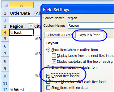
Create Indented Collapsible Row Excel Hierarchies To display more pivot table rows side by side, you need to turn on the Classic PivotTable layout and modify Field settings From the Excel Options menu choose Advanced then scroll down to the General section and press the Edit Custom List button From the Excel Options menu choose Advanced then scroll down to the General section and press the Edit Custom List button.
multiple fields as row labels on the same level in pivot table Excel - Microsoft Community
Smart Table Web Component | Table | Smart UI for ... - Smart UI Components Server-side Batch Edit; Server-side Cell Edit; Server-side CRUD; Server-side bind to MySQL DB; Server-side Grouping; Server-side Sorting; Server-side Filtering; Server-side Pagination with MySQL DB; Server-side Pagination; Server-side Tree Grid; Server-side Master Detail

How To Create A Pivot Table With Multiple Columns And Rows | Awesome Home
One Weird Trick for Smarter Map Labels in Tableau - InterWorks Set the transparency to zero percent on the filled map layer to hide the circles. Turn off "Show Mark Labels" on the layer with "circle" as the mark type to avoid duplication. If you don't want labels to be centered on the mark, edit the label text to add a blank line above or below. Experiment with the text and mark sizes to find the ...
.jpg)
Excel Pivot Tables Fields in Excel pivot tables Tutorial 02 June 2020 - Learn Excel Pivot Tables ...
excel table - Microsoft Tech Community In order to simplify the solution i adapted the table containing the allergens to this (This is done easily with IF function): The result would be like this with the main dish in horizontal order in rows 4 and 5 and the side dish in columns B and C: Mappe 56.xlsx. 39 KB.
Pivot Table Multiple Row Labels Side By Side | Decorations I Can Make
Self-Service Analytics - Gainsight Inc. The Field Display Name is the label that appears on your report. Activate Pivot reports by turning on the toggle. This toggle is only displayed if there are two or more fields under the Group By section. To know more about Pivot reports, refer to the Pivot section. Rename the chart labels in your reports using the Configure Aliases option.

Repeat all labels in an Excel pivot table | The Right Join
Excel Pivot Table Filters - Top 10 - Contextures Excel Tips In the Pivot Table, click the drop down arrow in the OrderDate field heading. In the pop-up menu, click Value Filters, then click Top 10. In the Top 10 Filter dialog box, change the number of Items to 5. Click OK, to close the Top 10 Filter dialog box, and apply the Value Filter.

Excel Pivot Table Tutorial & Sample | Productivity Portfolio
› excel-pivot-taHow to Create Excel Pivot Table (Includes practice file) Jun 28, 2022 · How to Create Excel Pivot Table. There are several ways to build a pivot table. Excel has logic that knows the field type and will try to place it in the correct row or column if you check the box. For example, numeric data such as Precinct counts tend to appear to the right in columns. Textual data, such as Party, would appear in rows.
Discover Pivot Tables – Excel’s most powerful feature and also least known
Improve Data Entry with Excel Data Forms - Productivity Portfolio Pin Excel Form on top of my worksheet with sheet name Five Main Differences with the Excel Forms. The form isolates one record or row.; Your orientation is vertical, not horizontal.; Some fields have keyboard shortcuts allowing you to jump within the form.; You have a series of Form buttons on the right-side to control navigation and filters.; The whole record is committed as opposed to each cell.
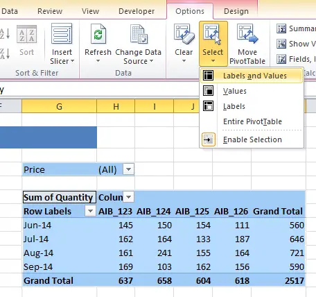
Excel Tip-How To Quickly Select All Or Just Parts Of Your Pivot Table - How To Excel At Excel
› pivot-table-tips-and-tricks101 Advanced Pivot Table Tips And Tricks You Need To Know Apr 25, 2022 · As a new pivot table user I LOVE this website – very well written! I do have a unique issue I’m hoping to get assistance with. I have a pivot table built out with multiple rows and columns pertaining to new hire information. My boss likes the option to “drill down” and view the source data.

Excel Pivot Tables: A Comprehensive Guide - HowToAnalyst
How To Round To The Nearest Tenth, Hundredth with Excel? The function MROUND. Another way to round to the nearest ten, five, etc. is to use the function MROUND. M stands for Multiple, where you set the argument to the nearest multiple you want to round to. For example, 10 if you want to round to the nearest ten or 5 to round to the nearest five. =MROUND (1234,10) =>1230.
Pivot Tables Excel 2007 Row Labels Side By | Brokeasshome.com
Excel: Merge tables by matching column data or headers - Ablebits Select any cell within your main table and click the Merge Two Tables button on the Ablebits Data tab: Make sure the add-in got the range right, and click Next: Select the lookup table, and click Next: Specify the column pairs to match, Seller and Product in our case, and click Next: Tip.

Excel Pivot Table Report - Sort Data in Row & Column Labels & in Values Area, use Custom Lists
How to Build Basic Reports (Horizon Analytics) - Gainsight Inc. The Field Display Name is the label that appears on your report. Activate Pivot reports by turning on the toggle. This toggle is only displayed if there are two or more fields under the Group By section. To know more about Pivot reports, refer to the Pivot section. Rename the chart labels in your reports using the Configure Aliases option.

Analyzing Data in Excel
xlookup: find sub categories and label with main category in new column Make a table of your data on sheet 1. Insert => Table After that copy the decription and paste them in column A of sheet VLookup. Make a table of your data on sheet VLookup Add manualy the Category. In Sheet 1 E2=VLookup(B2,Tabel2,2,0) After that a pivot table. Insert => Pivot Table. I filled the boxes on the right hand side with.
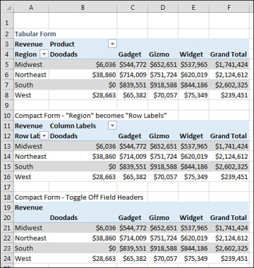
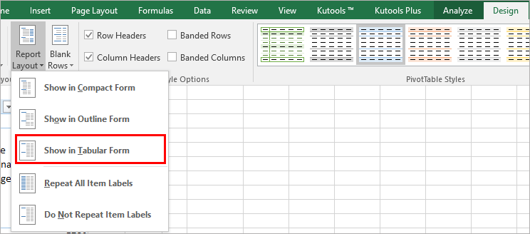
Making Report Layout Changes | Customizing a Pivot Table in Excel 2016 | InformIT
Excel Articles - dummies Articles 886. Cheat Sheet 19. Step by Step 162. Videos 10. Excel Excel 2010 All-in-One For Dummies Cheat Sheet. Cheat Sheet / Updated 04-20-2022. As an integral part of the Ribbon interface used by the major applications included in Microsoft Office 2010, Excel gives you access to hot keys that can help you select program commands more quickly.
How to make row labels on same line in pivot table?
PowerPoint Ribbon - Toolbars & Menus - BetterSolutions.com You can select menu commands by using the mouse or by using the keyboard. Pressing the Alt key will activate the Menu Bar an pressing the ESC key will deactivate the Menu Bar. You can move between the menus by pressing the Arrow Keys or the Tab key. You can expand a particular menu by pressing the Enter key or the Up or Down Arrow keys.

How to Sort Pivot Table Row Labels, Column Field Labels and Data Values with Excel VBA Macro ...
How to Group Data in Pivot Table (3 Simple Methods) Step 01: Navigate to Pivot Table. To start, click on the Insert ribbon at the top. Following, select the PivotTable drop-down and choose the From Table/Range option. Then, select the following options in the dialog box as shown in the picture below.
Repeat Pivot Table Labels in Excel 2010 - Excel Pivot TablesExcel Pivot Tables
How to convert rows to columns in Excel (transpose data) - Ablebits With the macro inserted in your workbook, perform the below steps to rotate your table: Open the target worksheet, press Alt + F8, select the TransposeColumnsRows macro, and click Run. Select the range that you want to transpose and click OK: Select the upper left cell of the destination range and click OK:
Post a Comment for "43 pivot table excel row labels side by side"