40 data labels excel pie chart

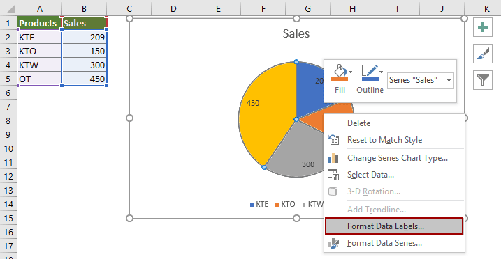
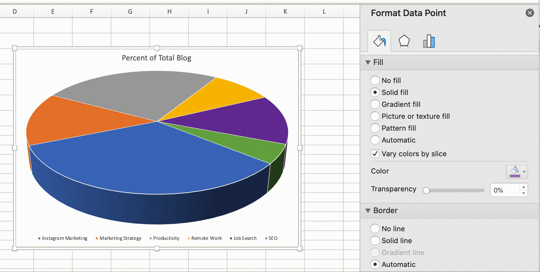
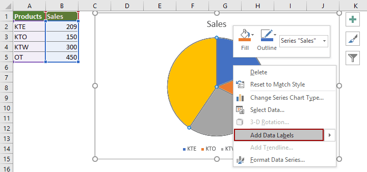
Change the format of data labels in a chart To get there, after adding your data labels, select the data label to format, and then click Chart Elements > Data Labels > More Options. To go to the appropriate area, click one of the four icons ( Fill & Line , Effects , Size & Properties ( Layout & Properties in Outlook or Word), or Label Options ) shown here. How to Make a Pie Chart in Excel & Add Rich Data Labels to ... Sep 08, 2022 · In this article, we are going to see a detailed description of how to make a pie chart in excel. One can easily create a pie chart and add rich data labels, to one’s pie chart in Excel. So, let’s see how to effectively use a pie chart and add rich data labels to your chart, in order to present data, using a simple tennis related example.

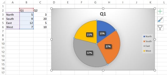
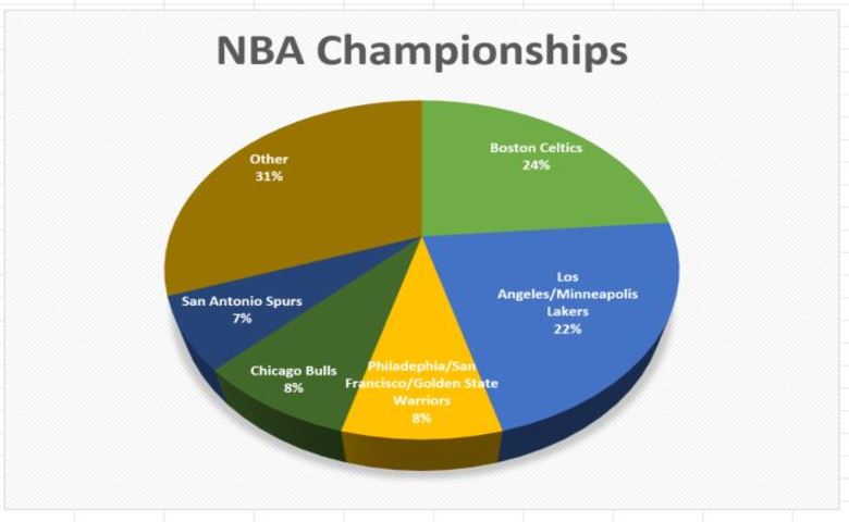
Add or remove data labels in a chart - support.microsoft.com Data labels make a chart easier to understand because they show details about a data series or its individual data points. For example, in the pie chart below, without the data labels it would be difficult to tell that coffee was 38% of total sales. Depending on what you want to highlight on a chart, you can add labels to one series, all the ...

Data labels excel pie chart

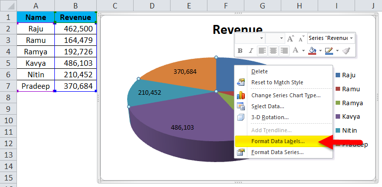
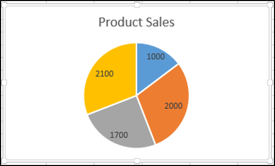
Create a Pie Chart in Excel (In Easy Steps) - Excel Easy 6. Create the pie chart (repeat steps 2-3). 7. Click the legend at the bottom and press Delete. 8. Select the pie chart. 9. Click the + button on the right side of the chart and click the check box next to Data Labels. 10. Click the paintbrush icon on the right side of the chart and change the color scheme of the pie chart. Result: 11. Pie Chart Examples | Types of Pie Charts in Excel with Examples It is similar to Pie of the pie chart, but the only difference is that instead of a sub pie chart, a sub bar chart will be created. With this, we have completed all the 2D charts, and now we will create a 3D Pie chart. 4. 3D PIE Chart. A 3D pie chart is similar to PIE, but it has depth in addition to length and breadth. How to Create Bar of Pie Chart in Excel? Step-by-Step The Bar of Pie chart is quite flexible, in that you can adjust the number of slices that you want to move from the main pie to the bar. Besides this, the Bar of pie chart in Excel calculates and displays percentages of each category automatically as data labels, so you don’t need to worry about calculating the portion sizes yourself.

Data labels excel pie chart. How To Make A Pie Chart In Excel. - Spreadsheeto How To Make A Pie Chart In Excel. In Just 2 Minutes! Written by co-founder Kasper Langmann, Microsoft Office Specialist. The pie chart is one of the most commonly used charts in Excel. Why? Because it’s so useful 🙂. Pie charts can show a lot of information in a small amount of space. They primarily show how different values add up to a whole. How to Create Bar of Pie Chart in Excel? Step-by-Step The Bar of Pie chart is quite flexible, in that you can adjust the number of slices that you want to move from the main pie to the bar. Besides this, the Bar of pie chart in Excel calculates and displays percentages of each category automatically as data labels, so you don’t need to worry about calculating the portion sizes yourself. Pie Chart Examples | Types of Pie Charts in Excel with Examples It is similar to Pie of the pie chart, but the only difference is that instead of a sub pie chart, a sub bar chart will be created. With this, we have completed all the 2D charts, and now we will create a 3D Pie chart. 4. 3D PIE Chart. A 3D pie chart is similar to PIE, but it has depth in addition to length and breadth. Create a Pie Chart in Excel (In Easy Steps) - Excel Easy 6. Create the pie chart (repeat steps 2-3). 7. Click the legend at the bottom and press Delete. 8. Select the pie chart. 9. Click the + button on the right side of the chart and click the check box next to Data Labels. 10. Click the paintbrush icon on the right side of the chart and change the color scheme of the pie chart. Result: 11.

5 New Charts to Visually Display Data in Excel 2019 - dummies

How-to Make a WSJ Excel Pie Chart with Labels Both Inside and ...

How to show percentage in pie chart in Excel?

information graphics - How to display data labels in ...

Create a Pie Chart in Excel (In Easy Steps)

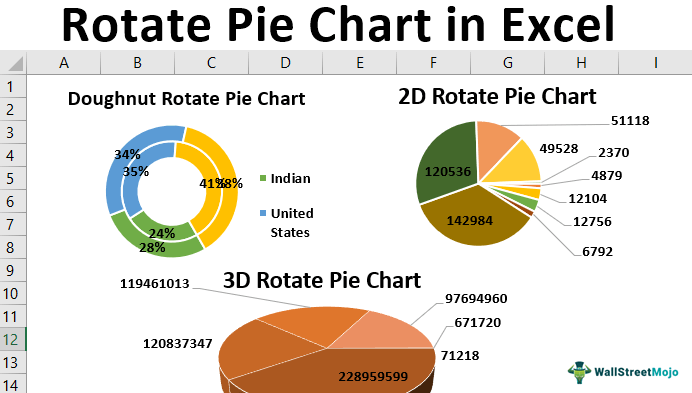
Rotate Pie Chart in Excel | How to Rotate Pie Chart in Excel?

Excel: How to not display labels in pie chart that are 0 ...

How to Show Percentage in Pie Chart in Excel? - GeeksforGeeks

How to Create a Pie Chart in Excel in 60 Seconds or Less

Automatically Group Smaller Slices in Pie Charts to one big Slice

Pie Chart in Excel | How to Create Pie Chart | Step-by-Step ...

How to Create a Pie Chart in Excel - Displayr

How to Make Pie Chart with Labels both Inside and Outside ...

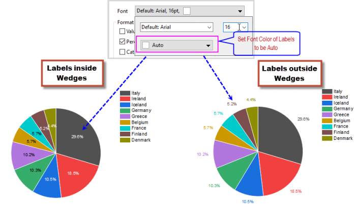
Help Online - Quick Help - FAQ-1019 How to customize the font ...

Solved: How can i see all data labels in a pie chart ...

How to Make Pie Chart with Labels both Inside and Outside ...

Help Online - Quick Help - FAQ-1017 How to recover the ...

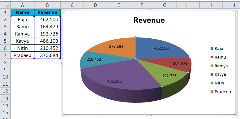
Adding data labels to a Pie Chart in VBA - Automate Excel

Office: Display Data Labels in a Pie Chart

Add data labels and callouts to charts in Excel 365 ...

Add or remove data labels in a chart

how to add data labels into Excel graphs — storytelling with data

Pie Chart in Excel | How to Create Pie Chart | Step-by-Step ...

Add or remove data labels in a chart

How to Make a Pie Chart in Excel

How to make a pie chart in Excel

How to Make an Excel Pie Chart

Create Outstanding Pie Charts in Excel | Pryor Learning

How to Data Labels in a Pie chart in Excel 2010

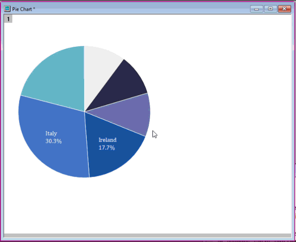
Change the format of data labels in a chart

How to: Display and Format Data Labels | .NET File Format ...

How to Make a Pie Chart in Excel - All Things How

How-to Add Label Leader Lines to an Excel Pie Chart - Excel ...

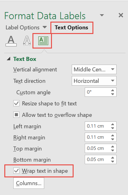
Is it possible to adjust the data label text box dimension in ...

How to show percentage in pie chart in Excel?

Microsoft Excel Tutorials: Add Data Labels to a Pie Chart

Add or remove data labels in a chart

How to fix wrapped data labels in a pie chart | Sage Intelligence

How to Create and Format a Pie Chart in Excel

How to fix wrapped data labels in a pie chart | Sage Intelligence

Share :