38 conditional formatting pivot table row labels
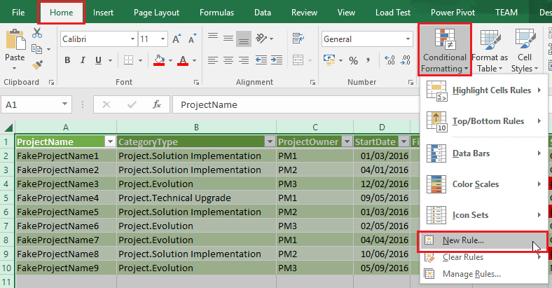
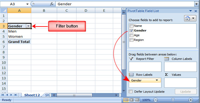
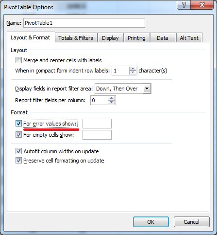
› pivot-table-calendarPivot Table calendar - Get Digital Help Apr 15, 2020 · The image above shows an empty Pivot Table placed on a worksheet, the task pane to the right allows you to quickly configure the Pivot Table. The task pane appears automatically when you select any cell in the Pivot Table and disappears when you go outside the Pivot Table. Go to a new sheet, I named it "Calendar". Go to tab "Insert" on the ribbon. Add Pivot Table Conditional Formatting and Fix Problems Mar 2, 2022 ... Fix Conditional Formatting Problem · Select any cell in the pivot table · On the Ribbon's Home tab, click Conditional Formatting, then click ...
Conditional Format Pivot Table Row | Chandoo.org Excel Forums If I change this apply this option to include the label row. I receive the following error: cannot apply a conditional format to a range that ...
Conditional formatting pivot table row labels
› excel-pivot-table-tutorialHow to make and use Pivot Table in Excel - Ablebits.com Sep 30, 2022 · It might be useful to create a Pivot Table and Pivot Chart at the same time. To do this, in Excel 2013 and higher, go to the Insert tab > Charts group, click the arrow below the PivotChart button, and then click PivotChart & PivotTable. In Excel 2010 and 2007, click the arrow below PivotTable, and then click PivotChart. community.powerbi.com › t5 › Community-BlogConditional Formatting Using Custom Measure - Power BI Sep 28, 2020 · Let us consider the following table visual: I have got sales by clothing category, by day of a week in the above table visual. Now, my task is to give a custom conditional formatting to the Day of Week column above based on the Clothing Category. For example - Clothing Category = Jackets should be GREEN. Clothing Category = Jeans should be BLUE Overwrite pivot table conditional format based on row label Apr 24, 2021 ... Overwrite pivot table conditional format based on row label · The formatting for the last 3 has the same colour for "fill" & "font" because I don't need the ...
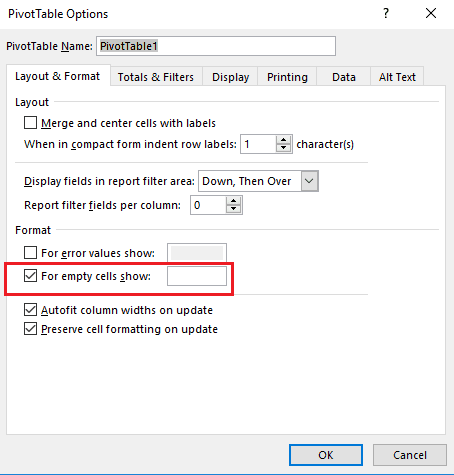
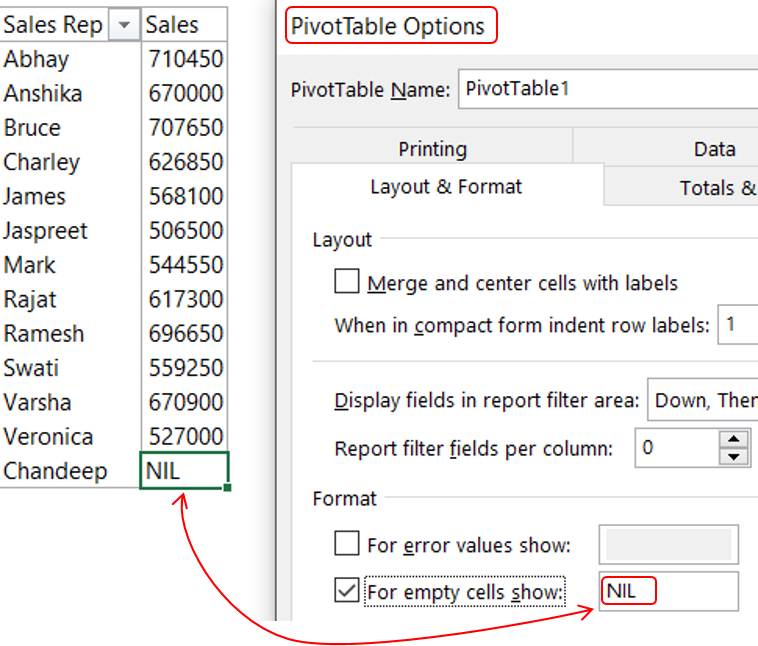
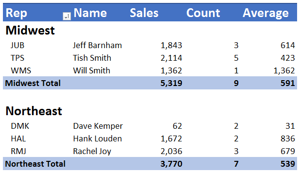
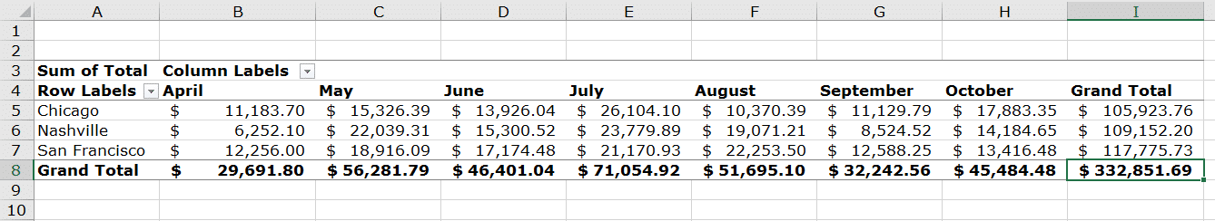
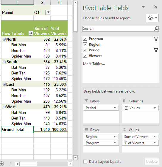
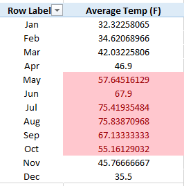
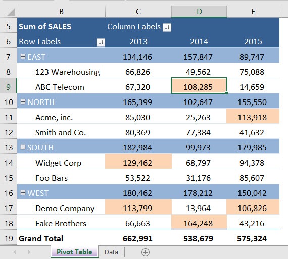
Conditional formatting pivot table row labels. How to Apply Conditional Formatting in Pivot Table? (with Example) To apply conditional formatting in the pivot table, first, we must select the column to format. In this example, select “Grand Total Column. › hide-blanks-excelHide Blanks in Excel PivotTables • My Online Training Hub Oct 11, 2018 · Pros: This setting is automatically applied to any new data added to your source that also contains empty cells.And if you add data to cells in your source data that were previously blank, the PivotTable will correctly update. i.e. the cells containing the space will be replaced with the new data upon refreshing the PivotTable. Conditional Formatting on Pivot Table row labels - Excel Help Forum Dec 31, 2012 ... It doesnt work. If i copy the powerpivot data to excel sheet and make it as source the conditional formatting under row label works. Any clues ... How to Apply Conditional Formatting to a Pivot Table in Excel 2. Apply Conditional Formatting on a Single Row in a Pivot Table · Select any of the cells. · Go to Home Tab → Styles → Conditional Formatting → New Rule.
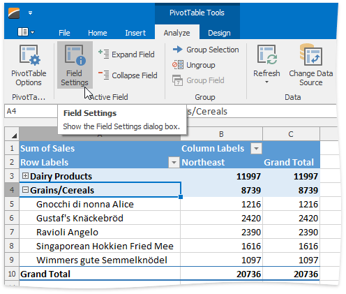
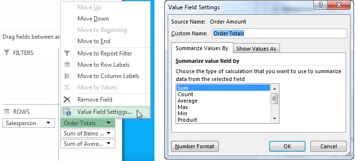
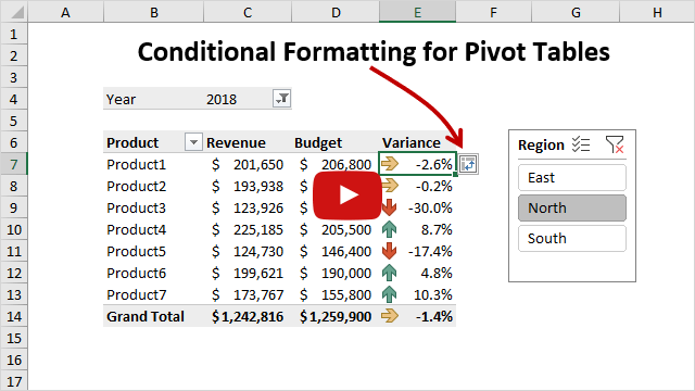
Automate Pivot Table with Python (Create, Filter and Extract) 22/05/2021 · Photo by Jasmine Huang on Unsplash. In Automate Excel with Python, the concepts of the Excel Object Model which contain Objects, Properties, Methods and Events are shared.The tricks to access the Objects, Properties, and Methods in Excel with Python pywin32 library are also explained with examples.. Now, let us leverage the automation of Excel report … How to Use Pivot Table Field Settings and Value Field Setting How to Refresh Pivot Charts | To refresh a pivot table we have a simple button of refresh pivot table in the ribbon. Or you can right click on the pivot table. Here's how you do it. Conditional Formatting for Pivot Table | Conditional formatting in pivot tables is the same as the conditional formatting on normal data. But you need to be careful ... In a pivot table, how to apply conditional formatting by label instead ... Jan 23, 2022 ... In a pivot table you can apply a conditional formatting to a group of value rather than to a cell or to the whole field thank to the ... Pivot Table Grouping, Ungrouping And Conditional Formatting Sep 29, 2022 ... Conditional formatting is used to define rules to format data values in the table. It helps us to identify the important data easily in a large ...
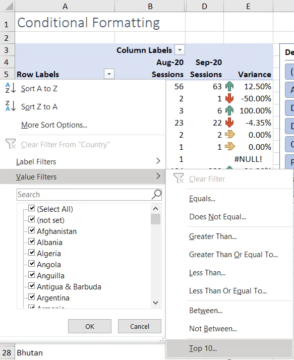
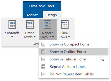
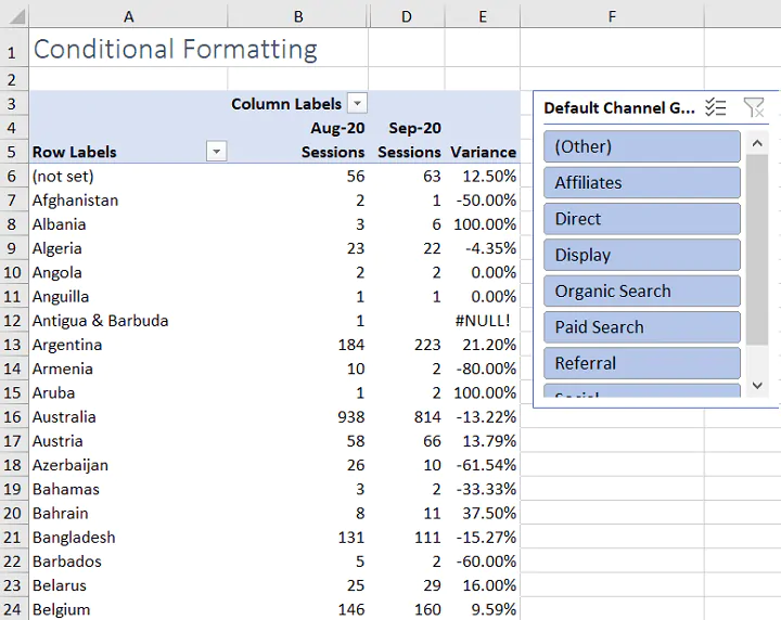
Highlight Cell Rules based on text labels - MyExcelOnline Nov 19, 2021 ... You can use conditional formatting with Excel Pivot Tables to highlight cell rules based on text labels. Click here to learn how! excelchamps.com › pivot-tablePivot Table Tutorial (100 Tips and Tricks) | Basic to Advanced When you add a pivot table with more than one item field you will get subtotals for the main field. But sometimes there is no need to show subtotals. In that situation, you can hide them using the following steps: Click on the pivot table and go to the Analyze tab. In the Analyze tab, go to Layout Subtotals Do not show subtotals. Design the layout and format of a PivotTable - Microsoft Support Change the way item labels are displayed in a layout form · In the PivotTable, select a row field. · On the Analyze or Options tab, in the Active Field group, ... community.powerbi.com › t5 › Community-BlogConditional Formatting in Power BI Tables The Color Based on and Summarization drop downs auto-populate the same filed name you wish to apply conditional formatting on. In order to customize or change the fields for formatting, a drop down containing the table names and field names will appear and you can choose the required field according to your requirement.
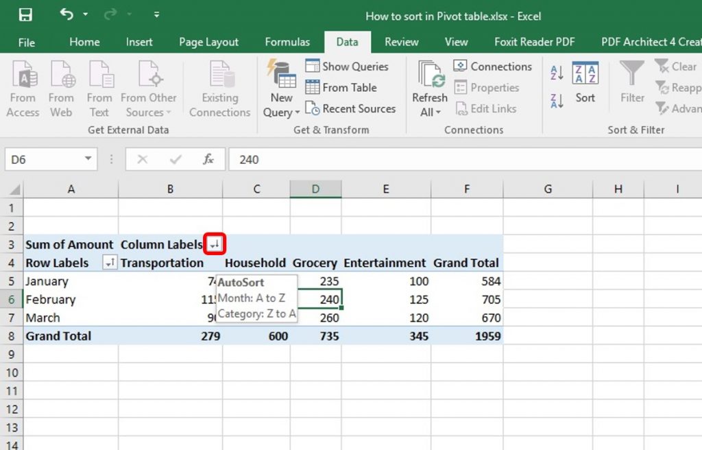
How to Sort Pivot Table | Custom Sort Pivot Table | A-Z, Z-A ...
support.microsoft.com › en-us › officeUse Excel with earlier versions of Excel - support.microsoft.com The conditional formatting rules will not display the same results when you use these PivotTables in earlier versions of Excel. What it means Conditional formatting results you see in Excel 97-2003 PivotTable reports will not be the same as in PivotTable reports created in Excel 2007 and later.
101 Advanced Pivot Table Tips And Tricks You Need To Know ...
Overwrite pivot table conditional format based on row label Apr 24, 2021 ... Overwrite pivot table conditional format based on row label · The formatting for the last 3 has the same colour for "fill" & "font" because I don't need the ...
Conditional Formatting in Excel - a Beginner's Guide
community.powerbi.com › t5 › Community-BlogConditional Formatting Using Custom Measure - Power BI Sep 28, 2020 · Let us consider the following table visual: I have got sales by clothing category, by day of a week in the above table visual. Now, my task is to give a custom conditional formatting to the Day of Week column above based on the Clothing Category. For example - Clothing Category = Jackets should be GREEN. Clothing Category = Jeans should be BLUE
Using ADF Pivot Table Components
› excel-pivot-table-tutorialHow to make and use Pivot Table in Excel - Ablebits.com Sep 30, 2022 · It might be useful to create a Pivot Table and Pivot Chart at the same time. To do this, in Excel 2013 and higher, go to the Insert tab > Charts group, click the arrow below the PivotChart button, and then click PivotChart & PivotTable. In Excel 2010 and 2007, click the arrow below PivotTable, and then click PivotChart.
How To Remove (blank) Values in Your Excel Pivot Table - MPUG

Unified Method of Pivot Table Formatting - yoursumbuddy
Pivot Table shows row labels instead of field name
Subtotal and Total Fields in a Pivot Table | DevExpress End ...

Pivot Table Conditional Formatting Weekend Data Highlight

10 Ways Excel Pivot Tables Can Increase Your Productivity ...
Formatting Tips for Pivot Tables - Goodly

Working with Pivot Tables – Sigma Computing
Dressing Up Your PivotTable Design
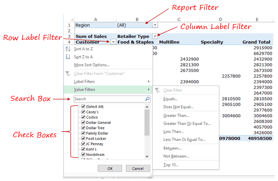
How to Filter Data in a Pivot Table in Excel
Group Items in a Pivot Table | DevExpress End-User Documentation
How to Apply Conditional Formatting to Pivot Tables - Excel ...
PivotTable Report Group Formatting - Excel University

How to Apply Conditional Formatting to Pivot Tables
How To Remove (blank) Values in Your Excel Pivot Table - MPUG
How to apply conditional formatting to Pivot Tables
Change the PivotTable Layout | EarthCape Documentation

Add Pivot Table Conditional Formatting and Fix Problems
How to Create a Pivot Table in Excel: Pivot Tables Explained
Lesson 54: Pivot Table Row Labels - Swotster
Pivot Table Conditional Formatting with VBA - Peltier Tech
Conditional Formatting for Pivot Table

Pivot Table Settings | JavaScript Spreadsheet | SpreadJS

How to Apply Conditional Formatting to a Pivot Table in Your ...
Hide #DIV/0! From Excel Pivot Table – Mike250
Excel Pivot Tables Explained • My Online Training Hub

How to add conditional formatting a Microsoft Excel ...

Conditional format a Pivot Table with the wizards ...
Pivot Table Conditional Formatting in Excel - GeeksforGeeks
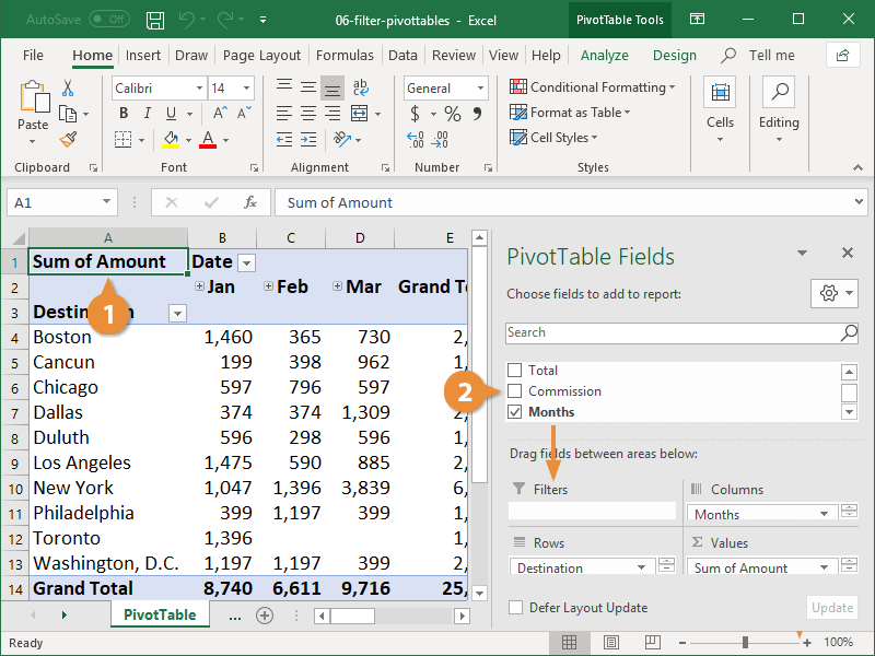
Pivot Table Filter | CustomGuide

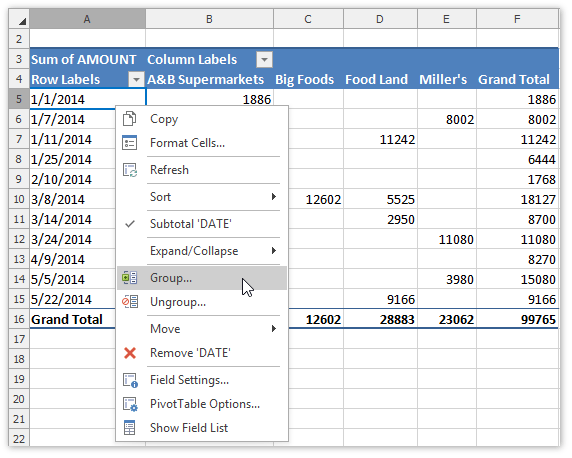
Pivot Table Grouping, Ungrouping And Conditional Formatting
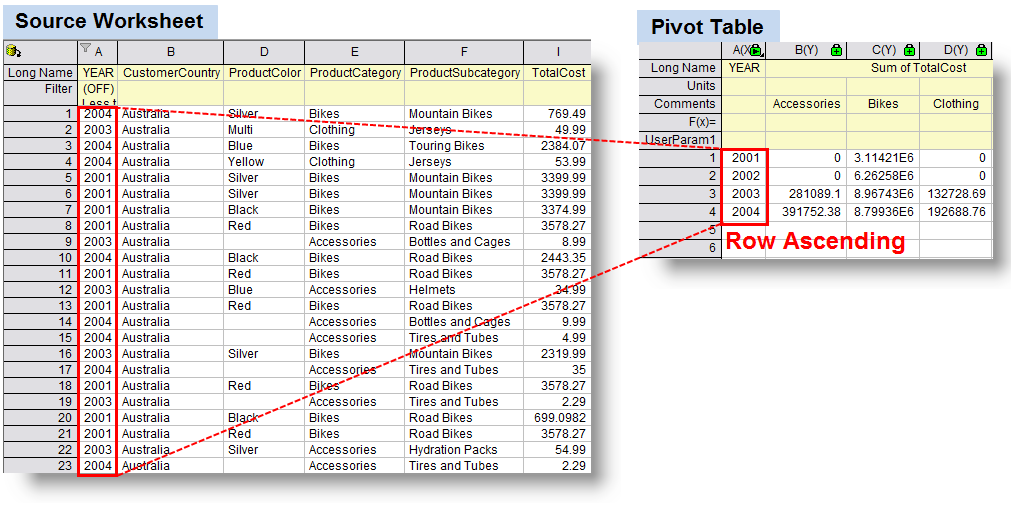
Help Online - Origin Help - Pivot Table
Conditional Formatting in Excel - a Beginner's Guide
Pivot Table Conditional Formatting | MyExcelOnline
Post a Comment for "38 conditional formatting pivot table row labels"